


How does normalisation work in Progenesis CoMet?
Normalisation is required in differential experiments to calibrate data between different sample runs. This corrects for factors that result in experimental or technical variation when running samples. For example, a common factor to correct for would be sample loading. The effect of these systematic errors can be modelled by a unique gain factor for each sample. The gain factor is represented by a scalar multiplier that is applied to each ion abundance measurement. The aim of normalisation is to determine the scalar factor αk for each sample which will allow us to recalibrate the sample to a normalisation reference run.
This can be modelled as follows:
y'i = αkyi
In other words, all compound ion abundances yi will be multiplied by the factor αk to give a normalised abundance y'i. There are several ways to calculate the scalar factor αk. Some common examples are (a) spiking in known quantities of metabolites and (b) using total metabolite abundance. All techniques will need to deal with technical variation that can bias the calculation of the scaling factor. In Progenesis CoMet we use a median and mean absolute deviation approach based on all the detected abundances to calculate the scalar factor. This is a more robust approach which is less influenced by noise in the data and reduces to a minimum any bias in the calculation.
To implement normalisation, we automatically select one run based on certain criteria that will mark it out as the most suitable reference for normalisation. Then, for each detected ion, we calculate a quantitative abundance ratio between the run being normalised and the reference run. The basic idea is that many compounds (and therefore compound ions) won't be changing in the experiment and so their quantitative abundance ratio should equal to 1. Due to experimental (or technical) variations such as differences in the quantity of sample loaded into the instrument, differences in ionization etc. the actual ratio will not be 1. Normalisation via the calculated scaling factor will correct for these experimental variations.
This correction can be done by calculating a robust distribution of all ratios and determine a global scaling factor. The distribution is calculated using the log of the abundance ratio values and as log(1) = 0.0 we expect to see the ratio distribution scattered about 0.0. Calculating in Log space ensures that up-regulation and down-regulation has the same weight.
For example, for a given ratio of 2/3 (a down regulation) and a ratio of 3/2 (the corresponding up-regulation), you find that log(3/2) = +0.176 and Log(2/3) = -0.176, so both are the same “distance” from 0 in log space. This is not the case in real space as 2/3 is closer to the desired ratio of 1 than 3/2 is and so would, incorrectly, be given a greater weight in calculating a mean ratio. We use the median and also use the median absolute deviation as an approximation of the mean and variance of the ratio distribution and we iterate this process to remove the influence of outliers. This gives a more robust estimation than just using the mean alone. The scaling factor is the anti-log of the mean of the log(ratios).
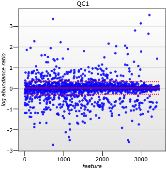
A scatter plot of log(abundance Ratio) after normalisation
In effect, you can think of each non-changing compound ion as a "spike" and this will result in potentially thousands of "spikes" across the dataset from which we can draw strength when determining the scaling factor. Instead of a handful of user chosen spikes we use all the experimental data resulting in a robust calculation.
A final point is that this approach to normalisation would be difficult, if not impossible, without prior high quality alignment and the detection of a single compound ion map that is then applied to all runs in the experiment, resulting in no missing values and 100% matching of data across all runs.