


How does normalisation work in Progenesis QI for proteomics?
Background
Normalisation is required in LC-MS proteomics experiments to calibrate data between different sample runs. This corrects for systematic experimental variation when running samples (for example, differences in sample loading). The effect of such systematic errors can be corrected by a unique gain factor for each sample - a scalar multiple that is applied to each feature abundance measurement. The key underlying assumption is that most peptide ions do not change in abundance (the abundance distributions do not alter globally), and hence recalibration to globally adjust all runs to be on the 'same scale' is appropriate.
This scalar factor required can be represented as for each sample:
Where is the measured peptide ion abundance of peptide ion on sample , is the scalar factor for sample and is the normalised abundance of peptide ion on sample .
However, there are several means by which this scalar can be estimated, even within the parameters of the key underlying assumption (that overall, the distributions do not change).
A commonly employed method to determine this scalar in the past was adjustment based on the total signal of all species in the sample (to total ion current, TIC); for example, expressing abundances as a proportion of the total. However, such a method is at risk of perturbation by changes in abundant species that dominate the total, and so can be inaccurate and introduce further variability.
Progenesis QI for proteomics instead uses ratiometric data in log space, along with a median and mean absolute deviation outlier filtering approach, to calculate the scalar factor. This is a more robust approach, which is less influenced by noise in the data and any biases owing to abundant species, as the absolute values of abundance are disregarded.
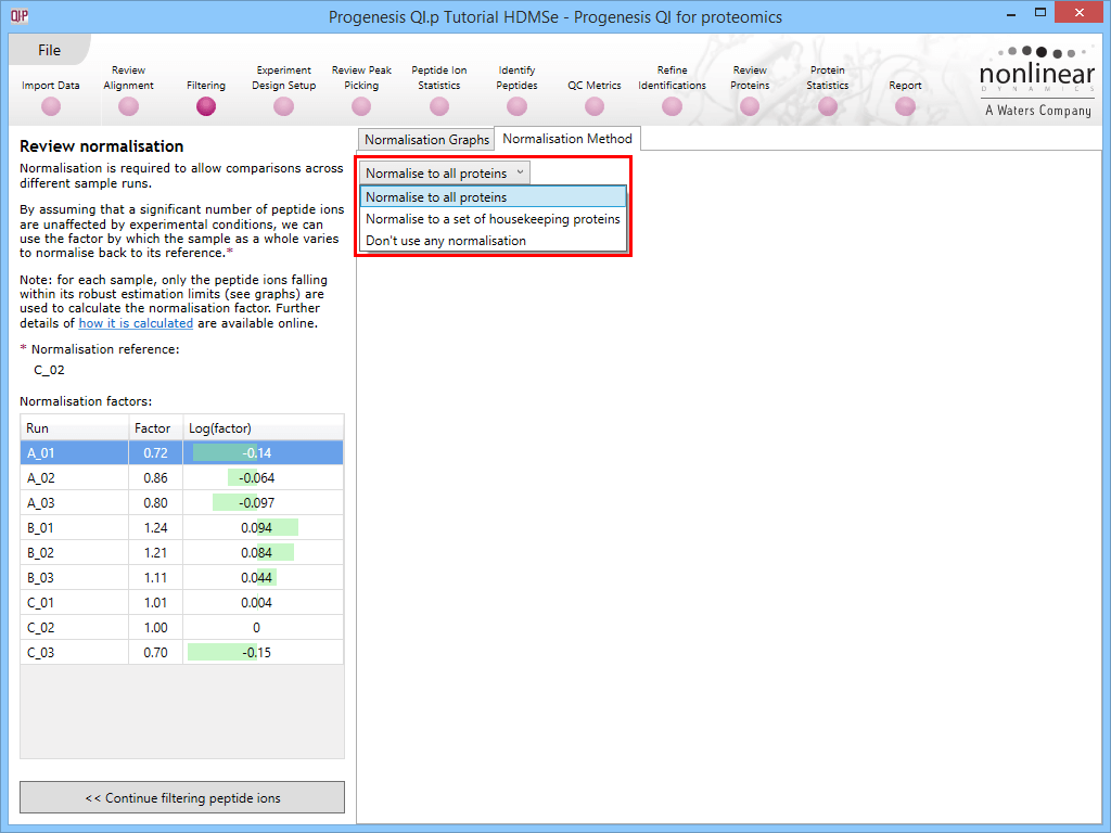
This default method is referred to as Normalise to all proteins at the Normalisation Method tab in the Review normalisation window at the Filtering stage of the workflow, and will be applied if no changes are made to the selection. There are two alternative methods available (Normalise to a set of housekeeping proteins and Don't use any normalisation) which will be covered later.
Process - Normalise to all proteins
Normalisation reference (the 'target')
One run is automatically selected as the normalisation reference (see detailed note [1]). Note that this may well not be the same as the alignment reference. Also, once selected, this run will not be re-evaluated if you add more runs to the experiment (so that your existing normalised data will not be altered).
Log10 ratio calculation
Because of the accurate alignment and aggregate co-detection, every run has a reading for all peptide ions. Hence, for every run, a ratio can be taken for the value of the peptide ion abundance in that run to the value in the normalisation reference:
Where is the ratio of the abundance of the peptide ion in run to that of peptide ion in the normalisation reference .
However, such ratiometric data follow a skewed distribution (a 2-fold increase giving 2, a 2-fold decrease giving 0.5; 3-fold giving 3 and 0.33, etc.). To obtain a distribution treating both directions equally, log transformation is applied, which yields a normal distribution. Progenesis QI for proteomics carries this transformation out (base 10) on all ratio data within each run, and for all runs, to generate a series of normal distributions. At this stage, these are offset – that is, because of scalar differences in signal, the ratios will not centre on 1 (and the log ratios not on zero), as would be the case if there was no global shift in the signal. This is the shift that must be addressed.
Note that this ratio calculation removes the influence of absolute abundance from the process, which is a major advantage over total-abundance-based methods.
Scalar estimation in log space
The next step is to centre the log10 ratio distributions onto that of the normalisation reference in each case. This is achieved by simply adding or subtracting the value required to shift the sample distribution over the normalisation reference one. This additive or subtractive shift in log space, is, of course, a multiplicative scalar in the sample abundance space.
There is a second improvement over traditional methods applied in this step. The median and also median absolute deviation are used as an approximation of the variance of the ratio distribution; this allows the filtering out of outlying ratio values so that they do not perturb the results. This process is carried out iteratively, to robustly remove the influence of outliers. See detailed notes [2] and [3].
Scalar application
Once the scalar has been derived in log space and then returned to an ‘abundance-space ratio’, it can be applied to all values in the sample run being normalised, and this completes the process.
Illustrations
The process as visualised in the software is shown below.
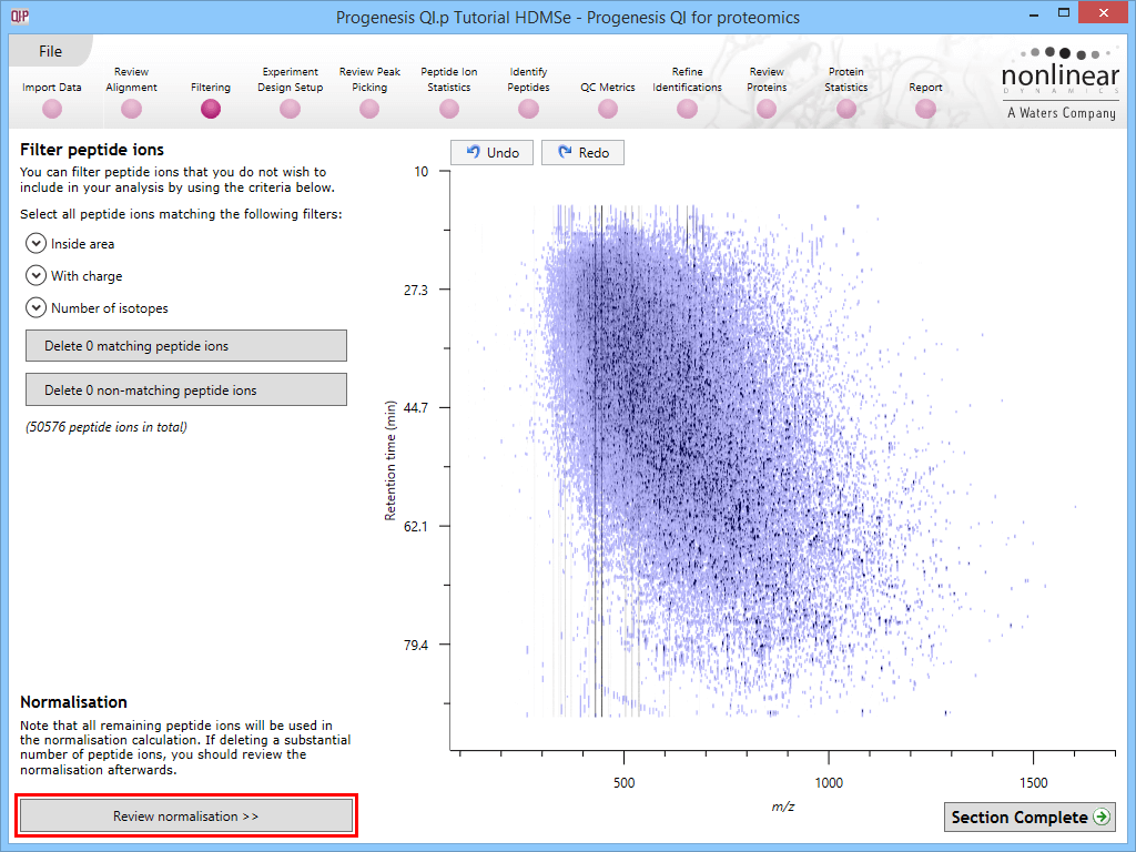
Select Review normalisation at the Filtering stage:
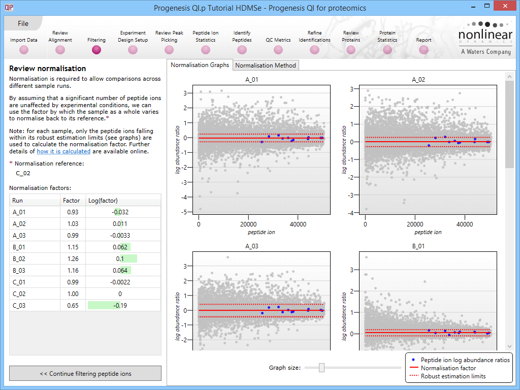
This will bring up the Review normalisation screen. The normalisation reference is indicated, and the log10 mean distribution shifts (the log10 scalars) are indicated in the table for each run.
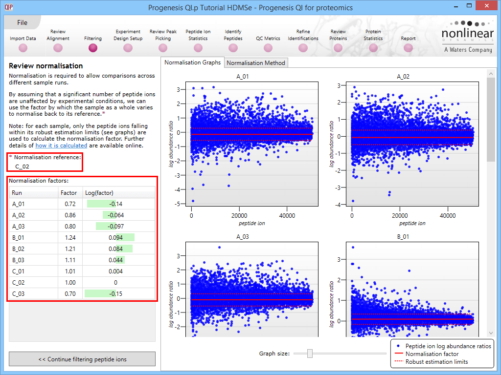
Detail for each run is shown on the right in the Normalisation Graphs tab, and the graph sizes can be adjusted using the slide-scale at the bottom of the page. The log abundance ratio is shown for each feature (ordered by ascending normalisation reference run abundance). The mean log abundance ratio and the robust estimation limits are shown as solid and dashed red lines. Hovering over a point will summon a tooltip with more information on that feature in that run and the normalisation reference, and hovering over the mean and robust estimation lines will provide more detail on their values.
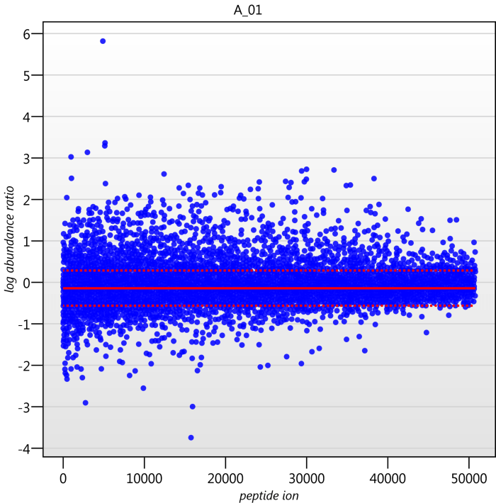
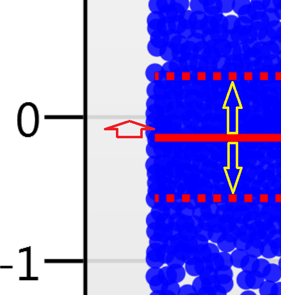
For the run above, the red arrow represents the normalisation shift required in log space, and the yellow arrows highlight the robust estimation limits.
Detailed notes
-
The normalisation reference is found by treating each sample as a putative normalisation reference, and calculating the robust standard deviation estimate (note [2]) for every other run. This set of standard deviation estimates is then used to calculate a pooled variance for each potential normalisation reference. The sample with the lowest pooled variance is used as the normalisation reference.
The pooled variance is not a measure of the 'total ratio distance' between one sample and all others, so that the scalar ratios you see may not be evenly 'up' and 'down'. Rather, it is a measure of how consistent its difference from all the other samples is across all the features. A sample that has a consistent scalar shift across all its analytes relative to another will introduce the minimum possible propagated error across all the analytes when they are scaled together (the scalar introduced in normalisation will be more accurate for more of the features, as more ratios are nearer to the mean value).
-
Median and Median Absolute Deviation (MAD) are used for outlier rejection before the robust mean and standard deviation estimates are calculated.
The upper and lower outlier limits are calculated as: Median + 3 * (1.4826*MAD)
Median – 3 * (1.4826*MAD)
Where 1.4826*MAD is an estimate of the standard deviation.The robust mean and standard deviation measures are then the mean and standard deviation of all of the log(abundance ratios) falling within these limits. The robust mean is used to calculate the normalisation scaling factor. This factor is 10^(-mean), converting back from a log shift to a scalar multiplier. The robust standard deviation is also used in the normalisation reference selection (as per [1] above).
-
Ions with an abundance of 0 for either the normalized or normalizing sample are not included in the calculation.
Alternative methods
Along with the Normalisation Graphs tab, one can also select the Normalisation Method tab at the Review normalisation screen. This provides access to two alternatives to the default (Normalise to all proteins is the default, as described previously).

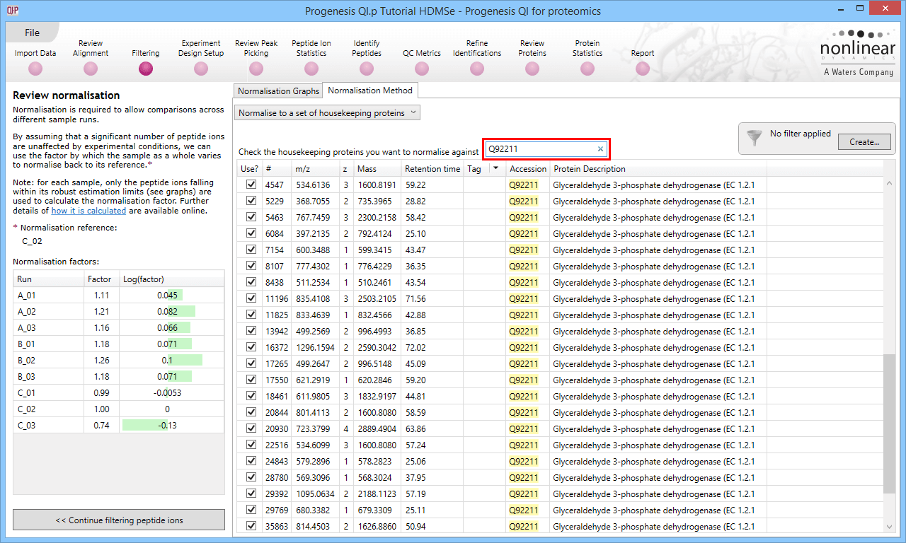
Normalise to a set of housekeeping proteins
This option allows you to normalise to either a 'spike' or to proteins you reasonably expect to be unchanging in the sample. It may be of benefit where the standard key assumption (that most species do not alter between samples) is known to be violated, so that the default method is no longer appropriate, but there are unchanging species present that can instead be used to standardise between the runs. Examples might include a dilution series with a consistent spike added where the bulk sample is being intentionally uploaded in sequence, or samples without any loading standardisation (so that variable amounts may be present) but with a consistently loaded spike. Alternatively, the assumption may be made that specific housekeeping proteins present in the sample will be unchanging despite the sample as a whole potentially altering. However, this application must be exercised with caution [ref 1].
If you wish to apply this option, naturally, you must first have identified your proteins to determine the peptide ions corresponding to your chosen standard.
There are then two ways to then select the appropriate peptide ions corresponding to that protein.
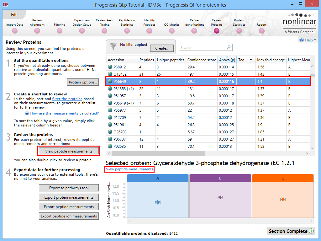
The first is to go to the Review Proteins stage, and in the table, find your standard(s) using the search box and their accession. Double-clicking on the relevant entry, selecting the View peptide measurements button on the left, or selecting the link below the table will bring up all the peptide ions comprising that protein. These can all be selected and tagged using the relevant column in the table.
Selecting a housekeeping protein's peptide ions by one of three methods.
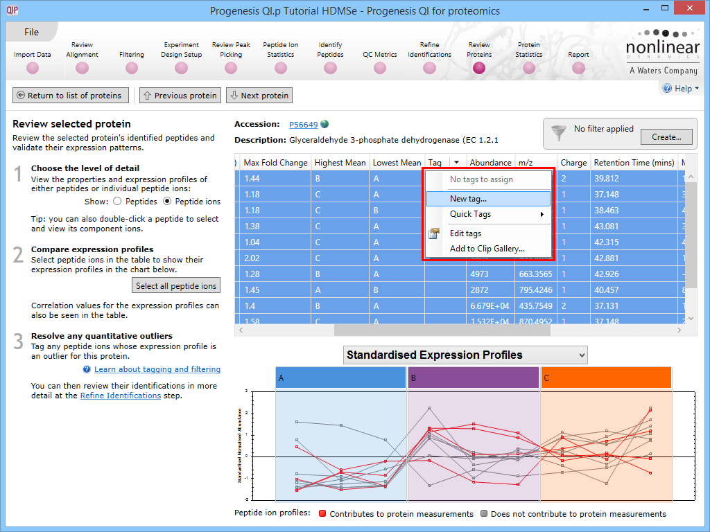
Tagging the peptide ions corresponding to the housekeeping protein.
Back at the Review normalisation stage in the Normalisation Method tab, the tagged peptide ions can be selected in the filter dialog. These can then all be selected and ticked, and on returning to the Normalisation Graphs, the housekeeping normalisation will be applied.
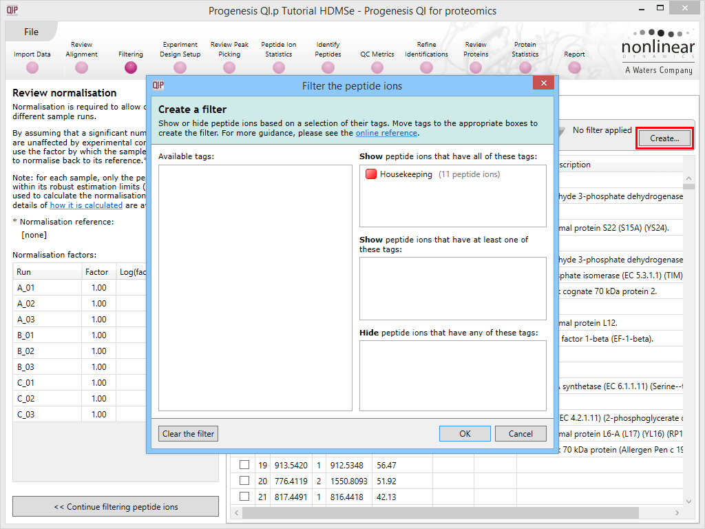
Applying a filter using the tag applied to the housekeeping peptide ions.
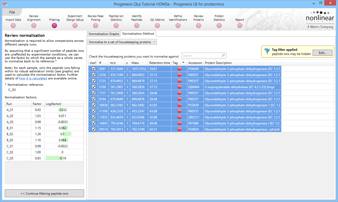
Selecting all the relevant peptide ions after filtering.
The restriction of peptide ion features used in the graphs can be seen on the updated plots, and the normalisation factors will also be updated.
The second method of setting the housekeeping protein is to simply search for its accession at the Review normalisation stage in the Normalisation Method tab directly, using the search box provided. Tagging is now optional, but the process is otherwise identical.
Reference
- Ferguson et al., 2005: "Housekeeping proteins: a preliminary study illustrating some limitations as useful references in protein expression studies." Proteomics 5 (2), 566-71.
Don't use any normalisation
Selecting this option will not apply any normalisation to the data (all representations and calculations will use raw abundance). This may be appropriate in certain specific cases, as determined by the user.