How do I use the Review Alignment screen?

Alignment is a key stage in the LC-MS workflow. It focuses on bringing all your LC-MS profile data into the correct alignment thus enabling a rapid and robust statistically driven analysis of the data. Typical workflows in alignment involve: either fully automatic or a combination of manual and automatic approaches to the addition of ‘alignment vectors’ to each image. The vectors correct for the distortion in the Retention time between each run and the chosen Reference run. This alignment facilitates accurate feature detection across the whole experiment.

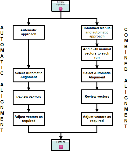
Alignment workflow

Alignment of LC-MS data runs can be approached either automatically or through a combination of manual and automatic approaches. An automatic approach is recommended followed by manual review of the alignment.

Fully automatic approach to alignment from Import Data

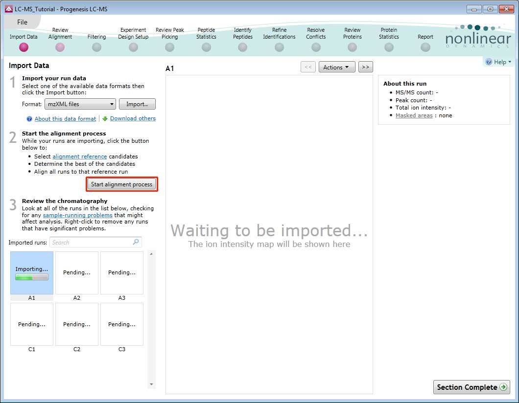
The Import Data stage incorporates the automated selection of the Reference Run and alignment of the runs in your data set to the Reference Run.

As the loading process starts, you can also start the automatic alignment before the loading has completed. This is a 2 stage process that involves the selection of an Alignment Reference (either automatically or manually) then the automatic alignment of all your runs to this Reference run.

Progenesis LC-MS provides three methods for choosing the alignment reference run, as seen below:

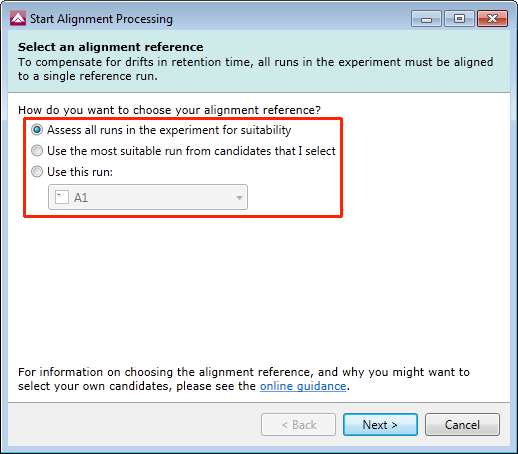
1. Assess all runs in the experiment for suitability

This method compares every run in your experiment to every other run for similarity. The run with the greatest similarity to all other runs is chosen as the alignment reference.

If you have no prior knowledge about which of your runs would make a good reference, then this choice will normally produce a good alignment reference for you. This method can take a long time.

2. Use the most suitable run from candidates that I select

This method asks you to choose a selection of reference candidates, and the automatic algorithm chooses the best reference from these runs.

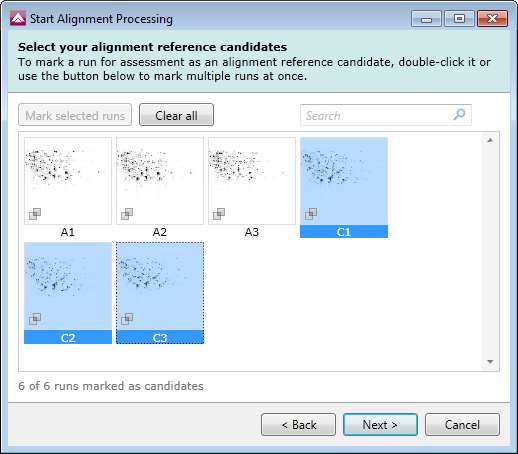
When you have some prior knowledge of your runs' suitability as references:

• runs from pooled samples
• runs for one of your experimental conditions will contain the largest set of common peptides

3. Use this run

This method allows you to manually choose the reference run.

Manual selection gives you full control, but there are a couple of risks to note:

• if you choose a pending run which subsequently fails to load, alignment will not be performed
• if you choose a run before it fully loads, and it turns out to have chromatography issues, alignment will be negatively affected (for this reason we recommend that you let your reference run fully load and assess its chromatography before loading further runs)

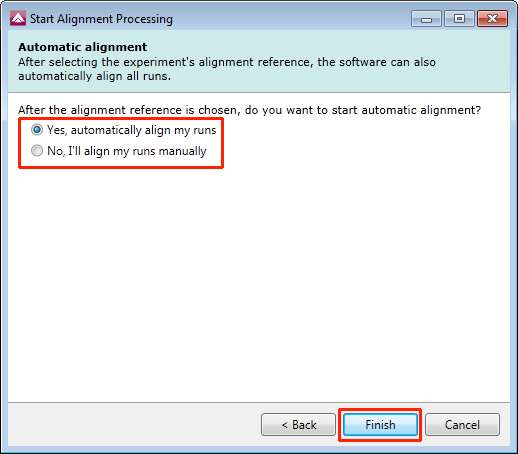
Once you have selected how to handle the choice of Reference run you will now be asked if you want to align your runs automatically or manually.

Select automatically and click finish.

Review Alignment

If you have selected the fully automatic alignment of your data then you will get a dialog informing you that you can Review alignment.

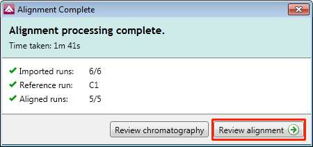
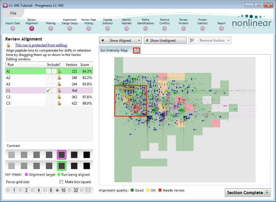
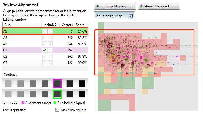
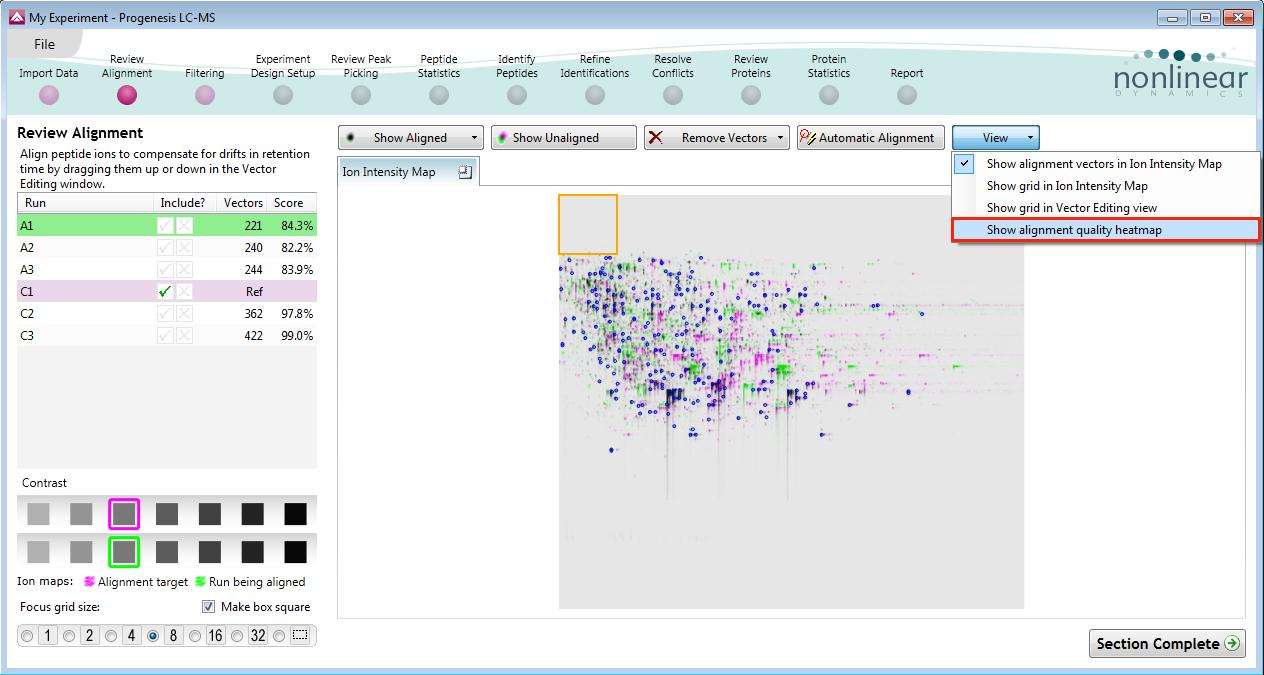
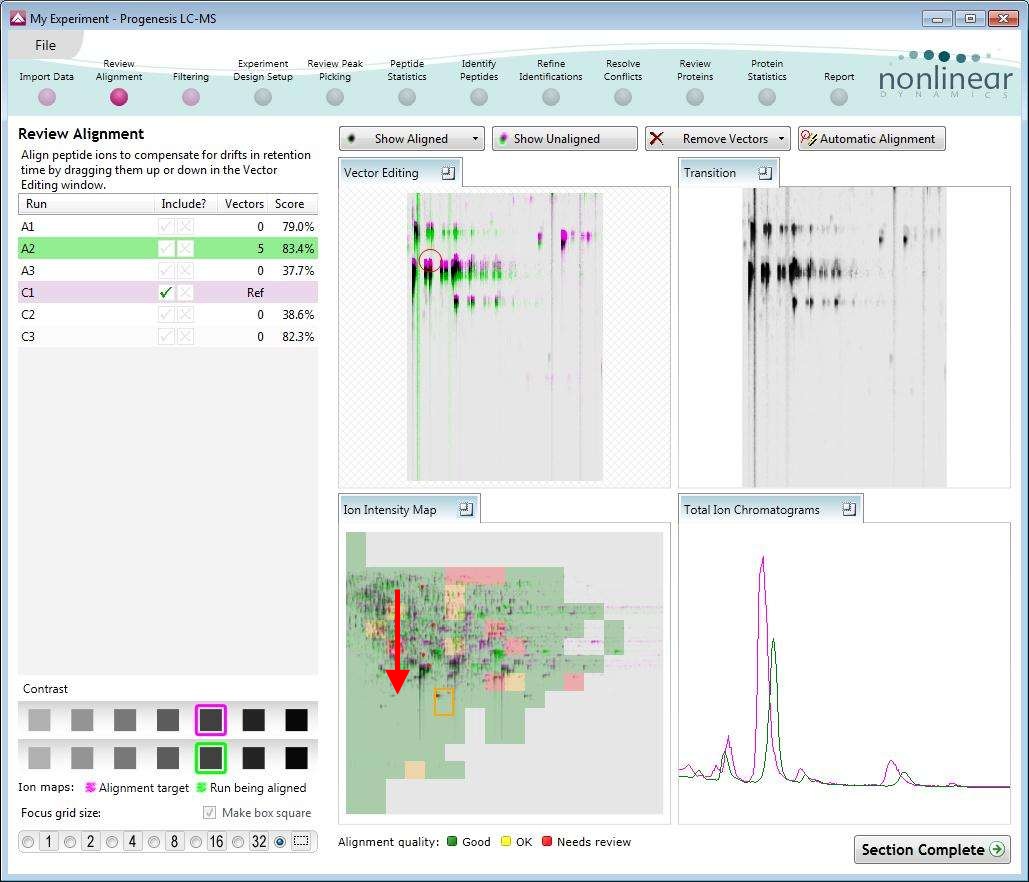
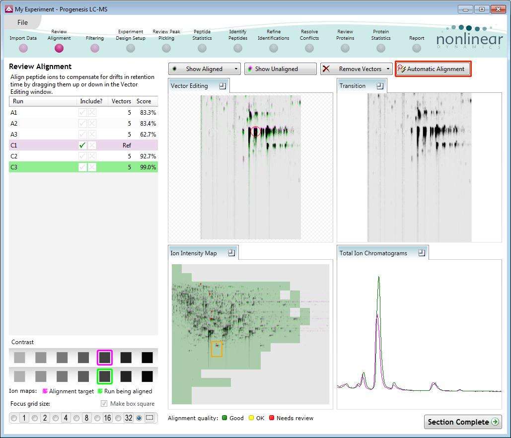
At this stage Progenesis LC-MS Alignment opens displaying the alignment of the runs to the Reference run (C1).

Layout of the Review Alignment step

To familiarize you with Progenesis LC-MS Alignment, this section describes the various graphical features used in the alignment of runs.

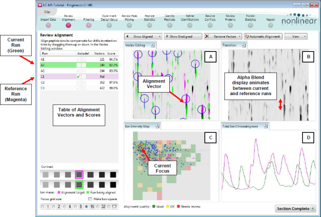
To setup the display so that it looks similar to the one above:

• In the Run table click on Run A2 to make it current. You will now be looking at the alignment of A2 to C1 in the Unaligned view.
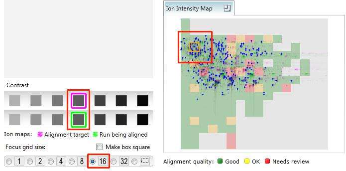
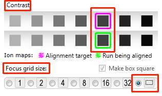
• Now adjust the size and position of the current focus. First select the size by clicking on the Focus grid size. Darken or lighten the runs using the contrast buttons. Then click on the Ion Intensity Map to ‘locate’ the current focus. The other 3 views will update to reflect the new focus.

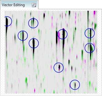
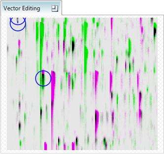
Vector Editing (Window A): is the main alignment area and displays the area defined by the current focus rectangle shown in Window C. The current run is displayed in green and the chosen reference run is displayed in magenta. Here is where you can review in detail the vectors and also place the manual alignment vectors when required.

Transition (Window B): uses an alpha blend to animate between the current and reference runs. Before the runs are aligned, the features appear to move up and down. Once correctly aligned, they will appear to pulse. During the process of adding vectors, this view will change to show a zoomed view of the area being aligned to help accurate placement of manual vectors.

Whole Run (Window C): shows the focus for the other windows. When you click on the view the orange rectangle will move to the selected area. The focus can be moved systematically across the view using the cursor keys. The focus area size can be altered using the controls in the bottom left of the screen or by clicking and dragging out a new area with the mouse. This view also provides a visual quality metric for the Alignment of the runs (note: this can be switched off using the options in the View menu) which focuses your review of the alignment process.

Total Ion Chromatograms (Window D): shows the current total ion chromatogram (green) overlaid on the Reference chromatogram (magenta). As the features are aligned in the Vector Editing view the chromatograms become aligned. The retention time range displayed is the vertical dimension of the Focus Grid currently displayed in the Whole Run view (Window C).

This view assists in the verification of the feature alignment.

Note: the icon to the right of the 'Window' titles expands the view.

Reviewing quality of alignment vectors

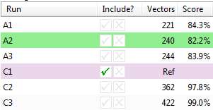
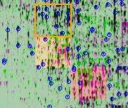
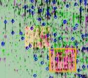
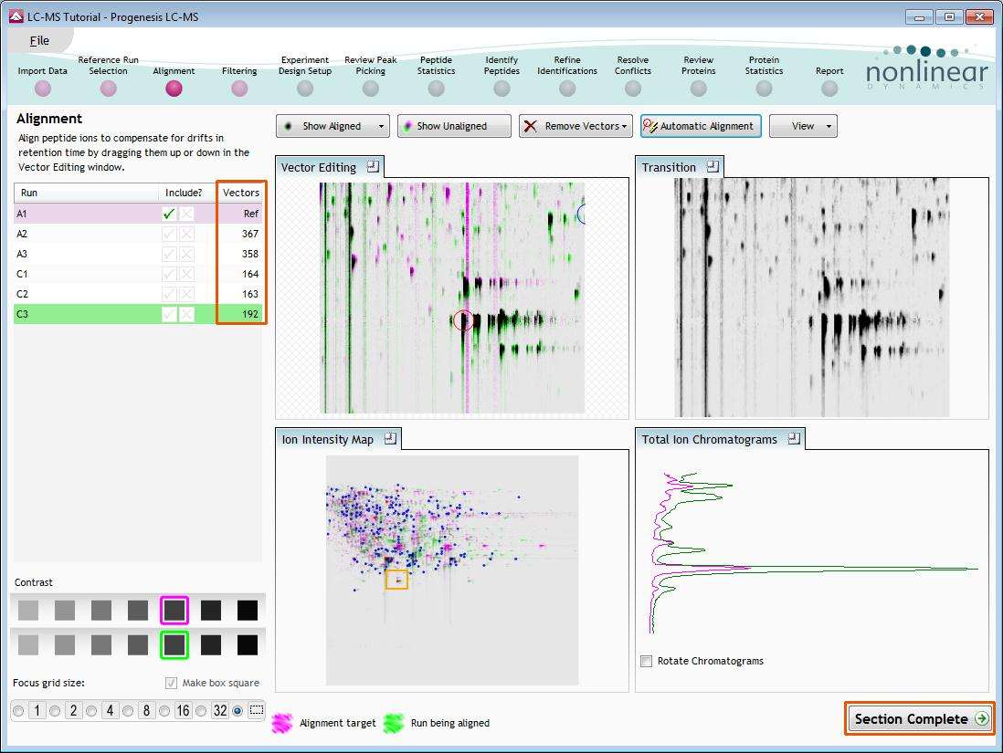
After Automatic alignment the number of vectors and Quality Scores will be updated on the Runs panel and the vectors will appear (in blue) on the view.

If the alignment has worked well then in Windows A and C the grid lines (option under View menu) should show minimal distortion, Window B (Transition) will show features pulsing slightly but not moving up and down.

Reviewing the quality of alignment

At this point the quality metric, overlaid on the Ion Intensity Map as coloured squares, acts as a guide drawing your attention to areas of the alignment. These range from Good (Green) through OK (Yellow) to Needs review (Red). When reviewing individual squares set the grid size to 16, (and untick the Make box square option) using the ‘Focus grid size’ control at the bottom left of the window. Three example squares are examined here.

For a ‘green’ square the majority of the data appears overlapped (black) indicating good alignment. When viewed in the Transition view the data appears to pulse.

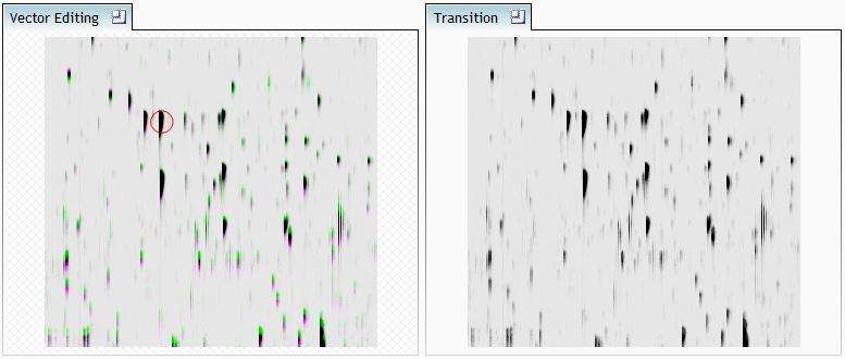
For a ‘yellow’ square some of the data appears overlapped (black) indicating OK alignment. When viewed in the Transition view some of the data appears to pulse.

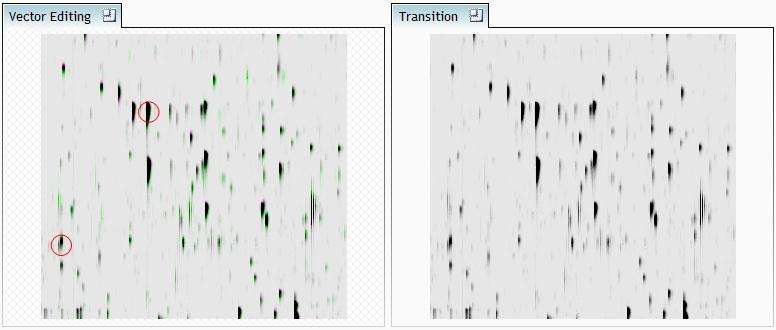
For a ‘red’ square little of the data appears overlapped (black) indicating questionable alignment. When viewed in the Transition view little data appears to pulse.

Note: the coloured metric should be used as a guide. In cases where there are a few ‘isolated’ red squares this this can also be indicative of ‘real’ differences between the two runs being aligned and should be considered when examining the overall score and surrounding squares in the current alignment.

The weighted average of the individual squares gives the overall percentage score for each run alignment.

Note: a marked red area combined with a low score clearly indicates a ‘miss alignment’ and may require some manual intervention.

Alignment scores

Before and after alignment of a run an Alignment score is shown in the Review Alignment table. This score is presented as the percentage of matchable peaks that are matched.

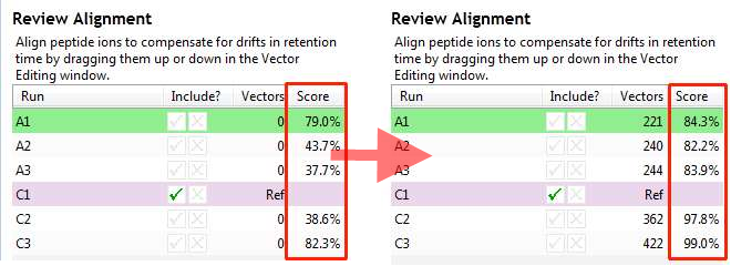
A match-able peak is a peak which does not look like noise and for which you can find a corresponding peak, with the same m/z, on the reference run within a defined time range. You then look how much of the peak intensity is overlapped by any aligned peak on the reference. Sum up the total matched intensity and the total match-able intensity which are used to give an aligned % for each of the little coloured squares.

The total % score, shown in the table, is then the weighted mean of the %score of each of the squares.

On the Ion Intensity Map the relationship between the coloured rectangles and the % score is:

• Red: < 33.3%
• Orange 33.3% to 66.6%
• Green > 66.6%

With regards to what the colour means with regards to relative alignment quality:

• Red: Needs Review
• Orange: OK
• Green: Good

Note: You can switch off the alignment quality heatmap using the option in the View menu

Combined manual and automatic approach to alignment

To place manual alignment vectors on your current run (A2 in this example):

1. Click on Run A2 in the Alignment panel, this will be highlighted in green and the reference run (A1) will be highlighted in magenta.
2. You will need approximately five alignment vectors evenly distributed from top to bottom for the whole run.
3. First ensure that the size of the focus area is set to 8 or Custom in the Focus grid size on the bottom left of the screen.



4. Adjust the dual contrast to suit.
5. Click on an area (see below) in the Whole Run window (C) to refocus all the windows. Adjust Contrast as required.

   

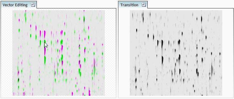
   Note: the features moving back and forwards between the 2 runs in the Transition view indicating the misalignment of the two runs.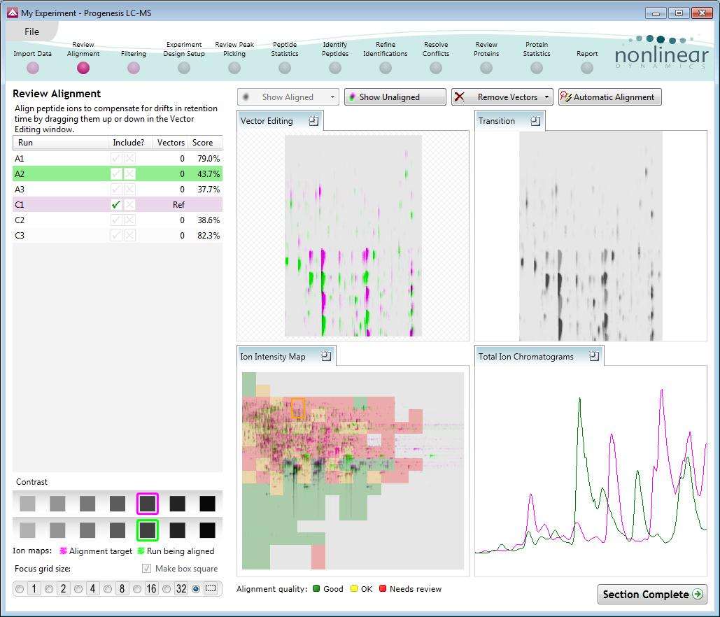
6. Click and hold on a green feature in Window A as shown below:

   

7. As you are holding down the left mouse button drag the green feature over the corresponding magenta feature of the reference image. The vector will appear as shown below as a red circle with a ‘cross hair’ indicating that a positional lock has been found for the overlapping features.

   

   Note: as you hold down the mouse button, window B zooms in to help with the alignment.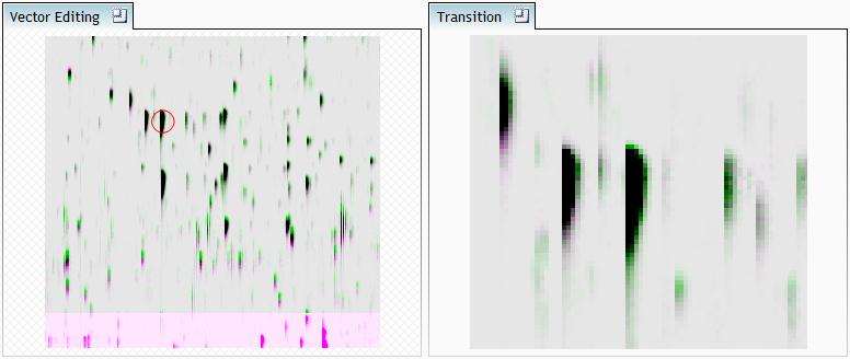
8. On releasing the left mouse button the image will ‘bounce’ back and a 'Red' vector, starting in the green spot and finishing in the magenta spot will appear.

   

   Note: an incorrectly placed vector is removed by right clicking on it in the Vector Editing window.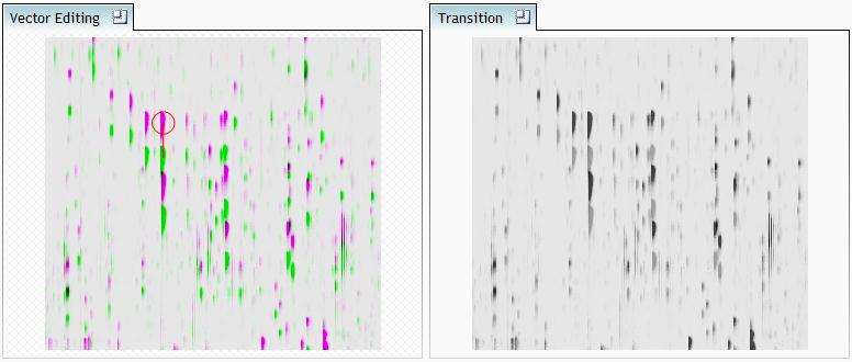
9. Now click Show Aligned on the top tool bar to see the effect of adding a single vector.

   

10. Adding another vector will improve the alignment further. Note this time as you click to add the vector it ‘jumps’ automatically to the correct position using the information from the existing alignment vector.

    

11. Repeat this process moving the focus from top to bottom on the Whole Run view. Note: the number of vectors you add is recorded in the Alignment table.

    

12. Now move on to the next run to align and repeat the addition of a few manual vectors.

    The number of manual vectors that you add at this stage is dependant on the misalignment between the current run and the Reference run. In a number of cases only using the Automatic vector wizard will achieve the alignment.

    Also the ‘ease’ of addition of vectors is dependent on the actual differences between the runs being aligned.

    Tip: When adding manual vectors to a run you may find it easier to switch off the quality heatmap using the option in the view menu.

    Note: On the addition of each manual vector the current quality score (%) will update, however the alignment will only update on the fly if you have the ‘Always Show Aligned’ selected in the Show Aligned menu.

13. Repeat this process, as required, for all the runs to be aligned.

    

14. Then select Automatic vectors and click OK.

    

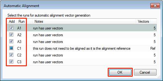
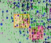
Note: the tick boxes next to the Run name control which files to generate vectors for. On completion, the number of vectors will be updated on the Alignment panel and the Automatic vectors will appear (in blue) on the image.

If the alignment has worked well then in Windows A and C the grid lines should show minimal distortion, Window B will show features pulsing slightly but with no movement of the features as it moves between the images.

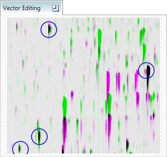
At this point, you should check the automatically placed (blue) vectors, as described on page 5 of this document. This will be easier with a larger grid size. Make sure the grid size is set to 4 using the ‘Focus grid size’ control at the bottom left of the window.

In each square, you can add additional manual vectors, if required. These will override any existing automatic vectors found at the same retention time. This increases the flexibility of the alignment, especially in regions where the misalignment/distortion arising from atypical chromatography appears complex.

Once alignment has been reviewed click Section Complete to start the Automatic Analysis of the aligned LC-MS runs.