


Principal Component Analysis
The Principal Component Analysis (PCA) in Progenesis QI uses compound abundance levels across runs to determine the principle axes of abundance variation. Transforming and plotting the abundance data in principle component space allows us to separate the run samples according to abundance variation. This is useful in identifying run outliers.
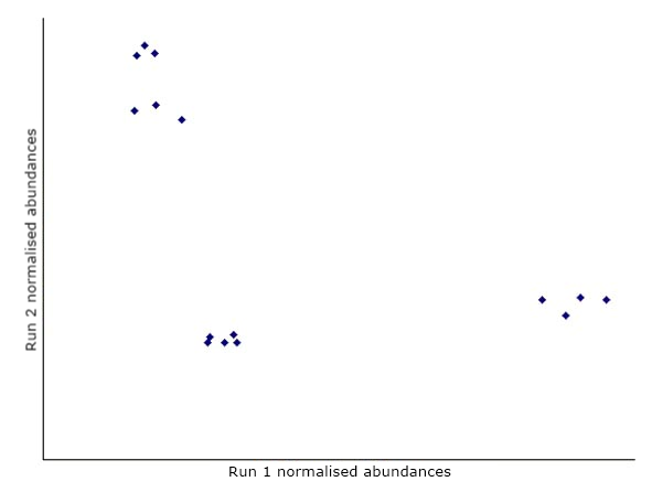
Consider a simple experiment with 2 runs and 15 compounds on each run. We can plot the normalised volumes of the compounds in a 2-dimensional graph:
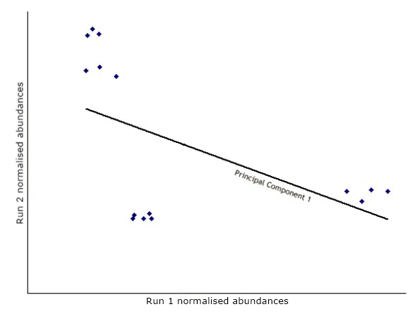
The first step in PCA is to draw a new axis representing the direction of maximum variation through the data. This is known as the first principal component.
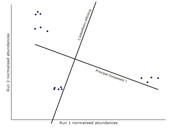
Next, another axis is added orthogonal to the first and positioned to represent the next highest variation through the data. This is the second principal component.
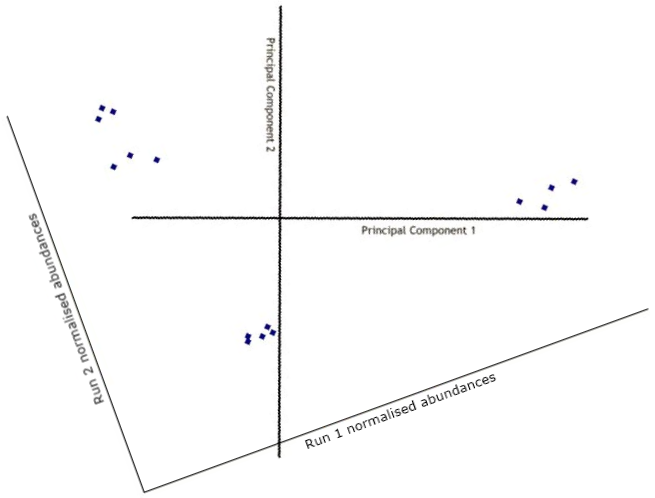
The data is then transformed (rotated) to view the points on the new axes.
Obviously, with just 2 runs this is fairly pointless, as our brains can quite easily see the relationships between points in a two-dimensional space. However, with 3 runs the points are plotted in a 3-dimensional space, with 4 runs the points are plotted in a 4-dimensional space, and so on. In these cases, the process of adding more principal components continues, each one orthogonal to the previous one and each one accounting for less and less of the variance in the data set.
The result of this is that we can visualise compounds (and runs) in two- or three-dimensional space in such a way that compounds that are "close together" (i.e. not showing much variation) will appear together on the PCA plot and vice versa. By displaying runs as well as compounds on the same graph (called a biplot), we can help show which compounds are contributing to the difference between runs. This can then be used to determine which compounds are most important in distinguishing a particular run or group from the other runs or groups.
The PCA biplot
We can graph both transformed compound and run data on a biplot. The biplot contains a lot of information and can be helpful in interpreting relationships between experimental groups and compounds. Also, it can help to identify outlier runs, i.e. runs that have different properties to other runs in the same groups. In the biplot shown below, we can see that runs from each group (the coloured dots) are close to each other. However, the runs in group "Drug C" (the orange dots) are not as close as the runs in the other three groups. The compounds are also shown and appear to form two distinct groups.
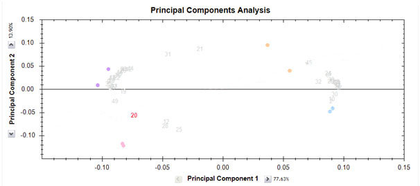
It is important to realise that if only those compounds that are significant (e.g. p-value < 0.05) are chosen, the PCA plot will be more likely to clusters runs according to their group. This is because a significant compound is one which exhibits differences between groups, and PCA captures differences between groups. Therefore, using significant compounds for the PCA will always see some sort of grouping. On the other hand, if we select all compounds and look at the biplot, we would still hope to see the groupings we expect. This can be a better indication of whether we have any run outliers. Finally, if all compounds are used in the biplot, it may be more useful to look at the second and third principle components. This is simply because PCA captures the variation that exists in the compound data and you have chosen all compounds. However, most of them will show no significant change (i.e. little variation) and so some other underlying source of variation may be captured in the first dimension.
Interpretation of compound position
The compound positions can be interpreted as follows. We can consider the compound number 20 in red on the biplot. Imagine a line going from the (0,0) position to the compound and also in the opposite direction. We can think of this as the compound axis. Like all axes, it has a positive side in the direction of the compound and a negative side in a direction away from the compound and on the other side of the (0,0) point.
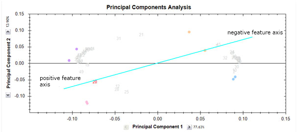
Now, runs on the positive side of the axis will have a high abundance value for the compound while runs on the negative side will have a low abundance value for this compound. The closer the run is to the axis, the more the influence of this compound for that run position. However, runs positions are determined by all compounds. Looking at the abundance profile we see that this is indeed the case.
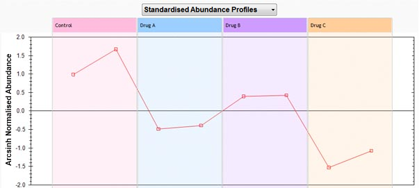
Drug C has a low abundance value for compound 20 while Drug A and Drug B have higher abundance values for the compound. So, in general we can say that compounds which are close to a run group on the biplot will have higher abundance value in this group than compounds further away. Also, compounds that are clustered together on the biplot should have similar abundance profiles and therefore should be clustered together in the dendrogram.